
The Gaussian splatting production workflow, from capture to publishing
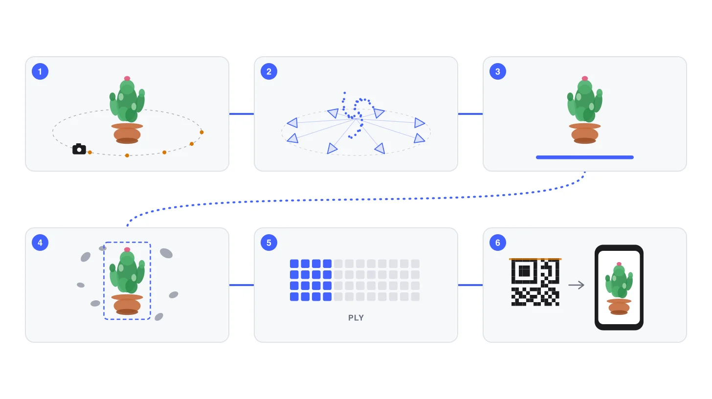
A Gaussian splat is the end of a chain. Photos go in at one end; at the other, a file light enough to open on a phone, from a link or a QR code, with the realism of a photograph. In between there are six stages, each with its own tools and its own ways of going wrong: capture, camera poses, training, cleaning, compression and publishing.
This article walks through them one at a time, as they are practised in 2026, with the sizes we measured on a real scene. If you are new to the technique itself, start with what Gaussian splatting is: here we assume you know that a splat is a cloud of small, soft, coloured ellipsoids learned from photos.
From photos to a published splat
Capture
Photograph or film the subject from every side, with plenty of overlap and settings that never change.
- In
- The subject, on a turntable or with room to walk around itA room with steady lightingA building or site, and a flight authorisation
- Out
- 50 to 200 photos for a small object — 427 for our cactus200 to 500 photos or more, or a slow videoThousands of aerial photos — 20,169 for a 3.7 km² campus
- Tools
- Mirrorless camera or phone, exposure locked; a turntableCamera, 360 camera or handheld LiDAR scannerMapping drone on an automatic flight plan, plus ground shots of the facades
- Time
- About 30 minutes1 to 2 hoursHalf a day or more
Camera poses
Work out where every photo was taken from, and a first, sparse cloud of 3D points.
- In
- The photosThe photos or video framesThe aerial photos, GPS/RTK positions, ground control points
- Out
- Camera positions and a sparse point cloudCamera positions and a sparse point cloudGeoreferenced camera positions
- Tools
- COLMAP, RealityScan, MetashapeCOLMAP, RealityScan — or the scanner’s own trajectoryDJI Terra, RealityScan, Metashape
- Time
- MinutesMinutes to an hourHours
Training
Optimise the Gaussians — position, shape, colour, opacity — until their render matches every photo.
- In
- Photos and camera positionsPhotos and camera positionsPhotos and camera positions
- Out
- A raw splat: 139,410 Gaussians, a 32.9 MB PLY for our cactus1 to a few million Gaussians, hundreds of MBTens of millions of Gaussians — 110 million on that campus
- Tools
- Postshot, LichtFeld Studio, Brush, gsplatThe same, with an exposure model for changing lightDJI Terra, Varjo Teleport, XGRIDS LCC Studio
- Time
- 15 to 40 minutes on a recent graphics cardOne to several hoursHours to days
Cleaning
Remove the floaters and everything that is not the subject; set the scale, the orientation, the colour.
- In
- The raw splatThe raw splat, sometimes several capturesThe raw splat
- Out
- The subject alone, upright and to scaleA clean room: floaters and veils gone, captures mergedA cropped, georeferenced site
- Tools
- SuperSplat in the browser, SplatTransform on the command lineSuperSplat, SplatTransformSplatTransform filters, SuperSplat, the drone software
- Time
- 15 minutes to an hour1 to 3 hoursHours
Compression
Make the file light enough to deliver: less colour detail, quantised values, sometimes levels of detail.
- In
- The clean PLYThe clean PLYThe clean PLY
- Out
- SPZ, 3.6 MB, or SOG, 4.4 MB — measured on our cactusA few tens of MB in SOG or SPZStreamed levels of detail: Streamed SOG, Spark RAD, 3D Tiles, LCC
- Tools
- SplatTransform, SuperSplat, PostshotSplatTransform, SuperSplatSplatTransform, Spark, Cesium, LCC Studio
- Time
- SecondsSeconds to minutesMinutes to hours
Publishing
Put the scene in front of people: a web page, an app, a headset, a game engine.
- In
- An SOG or SPZ fileA compressed fileStreamed tiles
- Out
- A viewer opened from a link or QR codeA tour with hotspots, in the browser or a headsetA digital twin in a map or an engine
- Tools
- PlayCanvas and SuperSplat, Spark (three.js), Babylon.jsThe same, plus Unreal Engine or Apple RealityKitCesiumJS, Cesium for Unreal, glTF
- Time
- HoursDaysDays to weeks
The six stages of a Gaussian splatting production, each with an animated drawing and four facts — what goes in, what comes out, the tools, the time — for three kinds of project: an object, an interior, a site flown by drone.
Pick a kind of project, then go through the stages: the facts change with the scale. The figures for the object are those of our cactus scene, captured by Steam Studio and published under CC0; the campus figures come from a Cesium demonstration; photo counts follow PlayCanvas’s capture guide. Times are orders of magnitude from those sources and from our own productions: they vary a great deal with the hardware and the care taken.
1. Capture: everything is decided here
No later stage can invent what the photos did not see. The capture is therefore where most of the quality — and most of the problems — are decided.
The rules are those of photogrammetry. Overlap: each photo should share 70 to 80% of its content with its neighbour on the same ring, and 60 to 70% with the ring above or below. Several heights: at least three rings of shots, from low to high, so that the top and underside of the subject are seen. Fixed settings: exposure, aperture, ISO, white balance and focus stay the same from the first photo to the last, which means manual mode. Sharpness: a shutter speed fast enough to rule out motion blur; recommendations range from 1/125 s to 1/500 s depending on the guide. And soft, even light: an overcast sky outdoors, diffused lights indoors.
How many photos? PlayCanvas suggests 50 to 100 for a small object, 100 to 200 for a medium one, 200 to 500 or more for a large scene. More is not always better: what counts is the variety of viewpoints, not the number of near-identical frames. Video works too, provided you extract the frames and discard the blurred ones.
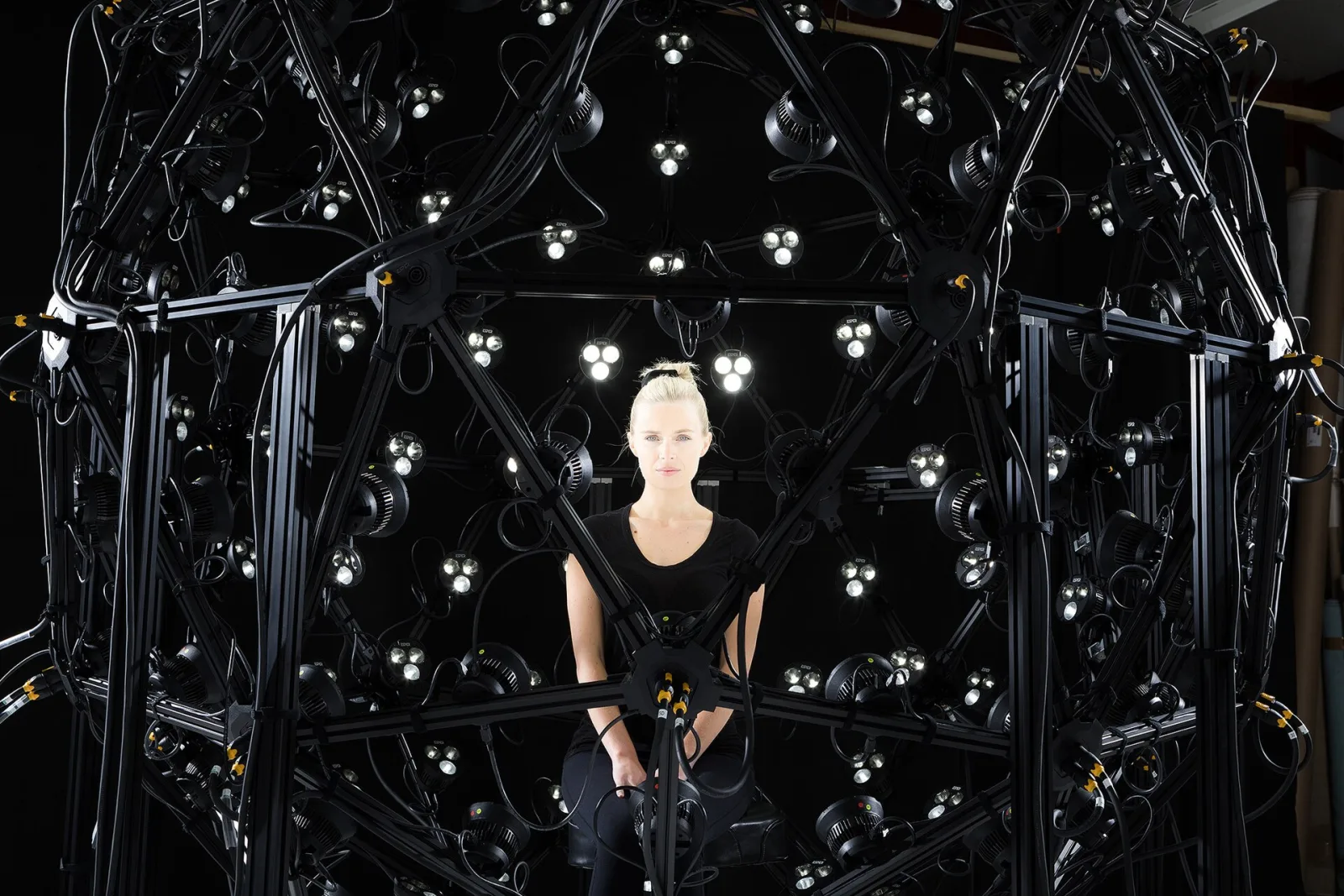
The most extreme version of a capture: a cage of synchronised cameras and lights that takes every viewpoint at once. For most projects, a single camera moved patiently around the subject does the same job, one photo at a time.
Image: ESPER HQ, CC BY 2.0, via Wikimedia Commons (resized, converted to WebP).The choice of device — phone, camera, 360 camera, handheld LiDAR scanner, drone — deserves an article of its own, and it is the subject of the next part of this series. It matters above all for what the capture guarantees, such as a true scale; we covered that in iPhone, 360 camera or LiDAR: what your capture guarantees.
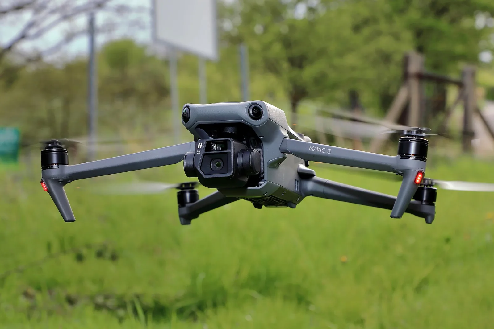
For a building or a site, the camera takes to the air. Drone mapping software now takes the photos straight into splat training — DJI Terra since version 5.0, in July 2025 — and Varjo Teleport, since May 2026, even flies the drone on an automatic plan.
Image: C.Stadler/Bwag, CC BY-SA 4.0, via Wikimedia Commons (resized, converted to WebP).2. Camera poses: where was each photo taken?
Before learning anything, the training must know, for every photo, where the camera stood and where it pointed. This is the job of structure from motion (SfM): the software finds the same details in several photos, then solves for the camera positions and a sparse cloud of 3D points at the same time. That cloud is the splat’s starting point: each point becomes a first Gaussian.
The reference tool is COLMAP, open source, which changed a great deal in 2026: version 4.0 (March) absorbed GLOMAP, a “global” method its authors found about an order of magnitude faster than the classic incremental one, as well as learned features; 4.1 (June) added GPU bundle adjustment and AMD cards. Commercial tools such as Epic’s RealityScan (formerly RealityCapture) and Agisoft Metashape solve the same problem and export their result in COLMAP format, which every splat trainer reads.
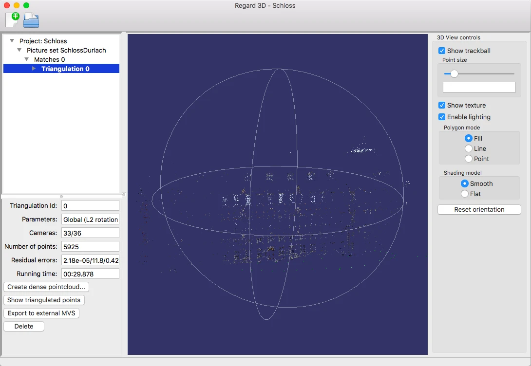
What structure from motion produces, here in the open-source Regard3D: 33 of the 36 photos placed, and 5,925 points outlining a castle facade. It is little — but enough to start training.
Image: Engelbert Niehaus, CC BY 4.0, via Wikimedia Commons (cropped, converted to WebP).A newer family of methods, led by VGGT (Meta and Oxford, CVPR 2025), estimates the cameras in a single pass of a neural network, in under a second. In 2026 they mostly show up in research pipelines and in captures with few photos; in production, COLMAP-style solvers are still the rule.
A handheld LiDAR scanner or a drone with RTK positioning simplifies this stage: the device already knows its trajectory, and the solver only refines it.
3. Training: the Gaussians learn
Training starts from the sparse cloud and adjusts, over tens of thousands of iterations, the position, shape, colour and opacity of every Gaussian, until the render from each camera matches its photo. Along the way it clones and splits Gaussians where detail is missing and removes those that serve no purpose; the first article in this series shows it step by step.
The desktop tools most used in 2026:
- Postshot (Jawset), commercial, Windows with an NVIDIA card; out of beta since August 2025, with plugins for Unreal Engine and After Effects.
- LichtFeld Studio, open source, NVIDIA; handles lenses with strong distortion and changes of exposure.
- Brush, open source, which runs almost anywhere — Mac, AMD, Android, even the browser — thanks to WebGPU.
- gsplat, the library behind Nerfstudio, for those who script their own pipeline.
On the phone, Scaniverse trains the splat on the device itself, in under 90 seconds, and Polycam does it in the cloud. For drones and scanners, the manufacturers’ software (DJI Terra, XGRIDS LCC Studio) or cloud platforms (Varjo Teleport) handle poses and training together.
How long does it take? On the Mip-NeRF 360 reference scenes, the gsplat library trains the standard 30,000 iterations in about 36 minutes on a TITAN RTX graphics card, using 5.7 GB of memory, and a scene capped at one million Gaussians in 15 minutes on an A100 (gsplat benchmarks). The settings that matter most are the maximum number of Gaussians — the newer “MCMC” trainers let you set it directly, which fixes the size of the file in advance — the number of iterations (around 7,000 for a preview, 30,000 for the final result) and the degree of spherical harmonics, which encode how the colour changes with the viewing angle.
Postshot’s May 2026 release, presented by its publisher: training profiles, region-of-interest training and the export formats.
Video: Jawset, on YouTube.4. Cleaning: what the training got wrong
A raw splat is never ready to show. Around the subject hang floaters, blobs the training created to explain an area it saw badly; the background, the ground, the operator’s feet are still there; the scene is tilted, off-centre, at an arbitrary scale.
The reference tool for this stage is SuperSplat, PlayCanvas’s editor, free, open source and running in the browser. You select Gaussians with a brush, a lasso, a box or a sphere, delete them without losing the undo history, merge several captures, correct the colour and set the orientation. Version 3.0, in September 2026, was rebuilt on WebGPU: it opens scenes of tens of millions of splats, and applies a colour correction to just a selection.
SuperSplat 3.0, presented by PlayCanvas in September 2026.
Video: PlayCanvas, on YouTube.For batch work, SplatTransform, from the same publisher, does it on the command line: crop to a box or a sphere, filter by opacity or size, remove floaters and isolated clusters automatically, merge, decimate. It is the tool we used to measure the sizes below.
5. Compression: from a hundred megabytes to a few
The raw file coming out of training is a PLY: 59 numbers per Gaussian, each stored on 4 bytes, so 236 bytes per splat. Of those 59 numbers, 45 describe how the colour changes with the angle (spherical harmonics of degree 3). A million splats weigh 236 MB; far too much to load on a phone.
Two families of formats solve this. SPZ, published by Niantic under the MIT licence, quantises each value on a few bits then compresses the whole; its version 4, in May 2026, encodes three to five times faster. SOG, open-sourced by PlayCanvas in September 2025, stores the Gaussians in WebP images the graphics card reads directly, with a palette for the colours. Rather than repeat the manufacturers’ ratios, we measured them.
What the scene weighs, format by format
Measured: our cactus, 139,410 splats
The same scene converted with PlayCanvas’s SplatTransform (v2.7.1). “SH 3” keeps the full view-dependent colour; “SH 0” keeps one colour per splat.
For comparison, the 427 original photos weigh about 7.8 GB — 236 times the raw PLY.
Estimate: your scene
Extrapolated from our two measured versions of the scene (139,410 and 204,684 splats). PLY and glTF are exact; SPZ and SOG are estimates.
Within the 1 million splats PlayCanvas recommends on phones.
Bar chart of the measured file sizes of one scene of 139,410 Gaussians in six formats, then a calculator that estimates each format’s size for a chosen number of splats and colour detail.
On our cactus, SPZ divides the raw PLY by 9 and SOG by 7 at full colour detail; dropping the view-dependent colour (SH 0) takes SOG to 1.8 MB, 18 times less. SOG gains less on a small scene because of its colour palette, about 2.3 MB in our measurements, which does not grow with the number of splats: on the scale of millions, the ratio climbs towards the “15 to 20 times” PlayCanvas announces. Compressed formats lose a little precision; the gain is almost always worth it.
Beyond a few million Gaussians — a building, a street, a site — a single file is no longer enough, whatever its format. The scene is then cut into levels of detail streamed according to the viewpoint, like the tiles of a map: Streamed SOG at PlayCanvas, the RAD format of Spark 2.0 (World Labs, April 2026), XGRIDS’ open LCC format, or 3D Tiles at Cesium, which streams 110 million splats covering 3.7 km².
And for exchanging files between tools, the standard is now glTF: its KHR_gaussian_splatting extension, carried by Khronos with Cesium, Esri, Niantic, NVIDIA and XGRIDS among others, was ratified in 2026. It defines where the data goes, not how to compress it; an SPZ compression extension is still being drafted.
6. Publishing: where people will see it
The last stage depends on where the scene will live.
- On the web, without an app: the PlayCanvas engine and its SuperSplat viewer, Spark for three.js, Babylon.js and CesiumJS all display splats in the browser, on a phone as on a computer. WebXR adds augmented and virtual reality on Android and in headsets.
- In a game engine: Unreal Engine through plugins (Postshot’s, Volinga, XScene), Cesium for Unreal for georeferenced scenes.
- On Apple devices: since WWDC 2026, RealityKit displays splats natively on iPhone, iPad, Mac and Vision Pro.
This is where the budget matters: PlayCanvas recommends about one million splats on a phone and three million or more on a computer. A scene that exceeds it must be streamed, or trained with a smaller budget from the start — which is why the cap on Gaussians is best set at stage 3.
How long does a project take?
Few independent figures exist. The studios that publish any agree on orders of magnitude: about a day for an object, a week for an interior, two to three weeks for a large exterior, and several more weeks when a custom viewer has to be developed (Utsubo, which sells these services: treat them as estimates). Machine time is now the smallest part: most of the time goes into preparing the capture, cleaning and integration.
Quality control: the six most common defects
Diagnose a defect
Floaters
- What you see
- Blobs or veils hanging in the air, especially in front of the camera path and indoors.
- Why
- Too few views of an area, or a surface the training could not explain: it “paints” with stray Gaussians.
- Prevented at
- Capture, then cleaning
- Fix
- More overlap when shooting; then select and delete them (SuperSplat), or filter them automatically (SplatTransform’s floater and cluster filters).
Blur off the path
- What you see
- Sharp from where the photos were taken, blurry as soon as you step away from that path.
- Why
- A splat only knows the viewpoints it saw. Between or beyond them, it guesses.
- Prevented at
- Capture
- Fix
- Shoot from several heights and all the way round; in the viewer, keep the camera within the captured zone.
Ghosts
- What you see
- Semi-transparent people, cars or leaves.
- Why
- Something moved during the capture: it is in some photos and not in others.
- Prevented at
- Capture
- Fix
- Shoot when the place is empty; mask moving objects in the photos before training; delete what remains.
Blotches
- What you see
- Patches of colour or brightness that shift from one angle to another.
- Why
- The exposure or the white balance changed between photos, or the light did.
- Prevented at
- Capture, then training
- Fix
- Lock the exposure, white balance and focus; train with an appearance model (for example the bilateral grid of LichtFeld Studio and gsplat).
Glass and mirrors
- What you see
- Reflections that float inside the object, transparent surfaces full of fog.
- Why
- A reflection moves with the viewpoint; the training explains it by putting Gaussians behind the surface.
- Prevented at
- Capture, then cleaning
- Fix
- Dull the reflections (polarising filter, matting spray where allowed) or hide the problem areas; this is still a research topic.
Holes
- What you see
- Parts missing: the top of an object, a ceiling, the underside of a table.
- Why
- No photo ever saw those surfaces.
- Prevented at
- Capture
- Fix
- Add a ring of shots from above (or below); for a site, add oblique drone passes and ground shots.
Six common defects of a Gaussian splat, each with an animated drawing and four facts: what you see, why it happens, the stage where it is prevented, and the fix.
Almost every defect is prevented at the capture, and almost none is fully repaired afterwards: cleaning removes what is wrong, it does not add what is missing. Hence the value of checking the photos — sharpness, overlap, exposure — before leaving the site.
Before delivery, a short checklist: the number of splats against the target device’s budget; the file size and the time before the first image appears; the colour detail kept (SH 0 to 3); floaters, from every angle the viewer allows; and, for large scenes, how the levels of detail behave when you move fast.
At ARGO
Everything we build runs in the browser, with no app to install, so the last two stages carry the most weight for us: a splat is only useful if it opens in a few seconds on the visitor’s phone, from a QR code on a package, a print or a stand. In practice, that means setting the budget of Gaussians from the capture, cleaning by hand, and delivering in a compressed format adapted to the target phones.
FAQ
Frequently asked questions
Sources and further reading
- PlayCanvas, Taking photos for Gaussian splatting · Performance and splat budgets · SOG format · SuperSplat 3.0 · SplatTransform
- COLMAP changelog · Pan et al., Global Structure-from-Motion Revisited (GLOMAP), arXiv:2407.20219 · Wang et al., VGGT, arXiv:2503.11651
- Kerbl et al., 3D Gaussian Splatting for Real-Time Radiance Field Rendering, SIGGRAPH 2023 — arXiv:2308.04079 · gsplat benchmarks · Kheradmand et al., 3D Gaussian Splatting as Markov Chain Monte Carlo, arXiv:2404.09591
- Niantic Spatial, SPZ 4 · Khronos Group, KHR_gaussian_splatting · World Labs, Spark 2.0 · Cesium, 3D Gaussian splats with levels of detail
- The scene measured in this article: Steam Studio, cactus sample data, CC0 — steam-studio.jp
Figures and statuses checked in September 2026. File sizes measured on 30 September 2026.